Next: ITRULE Algorithm:
Up: Rule inference
Previous: Formal Definition:
To search for `interesting' rules we need a preference measure to rank the rules and
an algorithm which uses the preference measure to find the `best' rules.
In general, the conditional probability, also called
``transition probability'' or ``confidence'' is a
belief parameter associated with every rule:
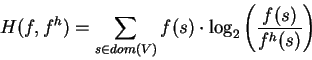
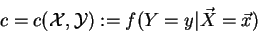 |
(26) |
It expresses the percentage for which the rule-implication is actually true.
Another measure, mostly used for association rules (see below), is ``support''.
It expresses the significance of a rule by measuring the probability that the
true implication of the rule occurs in the data:
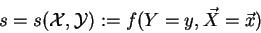 |
(27) |
An interesting information theory based measure for general rule induction was
introduced in 1988 by Goodman and Smyth [13]. The ``J-measure''
is a mixture of the probability of
 and a special case of
Shannon's cross-entropy. As a refresher, cross-entropy or directed divergence, is
defined as (section 3.3.2, [28, pg. 279], [38, pg. 12]):
and a special case of
Shannon's cross-entropy. As a refresher, cross-entropy or directed divergence, is
defined as (section 3.3.2, [28, pg. 279], [38, pg. 12]):
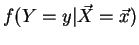
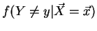
In rule-inference we are interested in the distribution of the the
``implication'' variable Y,
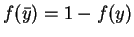
and especially in its two events y and complement  .
We want to measure the difference between
the a priori distribution f( Y), i.e. f(Y=y) and
.
We want to measure the difference between
the a priori distribution f( Y), i.e. f(Y=y) and
 ,
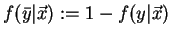
and the a posteriori
distribution
,
and the a posteriori
distribution
 ,
i.e.
,
i.e.
 and
and
 .
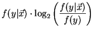
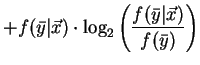
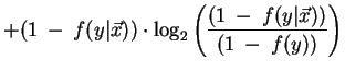
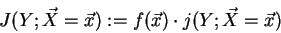
The ``j-measure'' (small j) is defined as ``the average mutual information between the events
(y and )
with the expectation taken with respect to the a posteriori probability
distribution of (Y).'' [41, pg. 304]. Denote
.
The ``j-measure'' (small j) is defined as ``the average mutual information between the events
(y and )
with the expectation taken with respect to the a posteriori probability
distribution of (Y).'' [41, pg. 304]. Denote
 and
and
 :
:
This measure is maximized when the ``transition''-probability
equals 1 (or 0), and minimized (=0) when the transition-probability equals the a priori
probability f(Y=y). ``In this sense the j-measure is a well-defined measure
of how dissimilar our a priori and a posteriori beliefs are about (Y) --
useful rules imply a high degree of dissimilarity." [41, pg. 305].
Summarizing, the j-measure includes two important features. The first is the ``goodness of fit''
between the rule hypothesis and the data, expressed by
having maximal values for transition probabilities
close to 1 (or 0 for a negative rule).
Second is the amount of ``dissimilarity'' compared with the unconditionalized
distribution. A rule with similar confidence
as the overall conclusion probability,
 ,
wouldn't make much sense, even if that
probability is close to 100%. As an example imagine 90% of all customers buy milk, then a
rule ``buying bread
,
wouldn't make much sense, even if that
probability is close to 100%. As an example imagine 90% of all customers buy milk, then a
rule ``buying bread
 buying milk with c=91%'' wouldn't be very useful.
The implication of buying milk is not given by buying bread,
it is just a general pattern.
buying milk with c=91%'' wouldn't be very useful.
The implication of buying milk is not given by buying bread,
it is just a general pattern.
A third feature is ``simplicity'' which is combined with the j-measure to form the
J-measure. Simplicity is a measure for the complexity of a rules precondition.
The more likely the truth of the precondition, the simpler and more
useful the rule. But the likelihood of the precondition is just the probability
 .
Therefore the average information content of a rule can be defined as:
.
Therefore the average information content of a rule can be defined as:
 |
(29) |
Next: ITRULE Algorithm:
Up: Rule inference
Previous: Formal Definition:
Thomas Prang
1998-06-07